LQSGW+GRISB calculation of FeSe
In this example, we illustrate how to perform LQSGW+GRISB calculation of FeSe.
LQSGW calculation of FeSe
For convenience, we prepared the input file ini for LQSGW calculation in the folder lqsgw. Starting with folder 4_FeSe, One could calculate by typing the following command or prepare your job file accordingly and submit:
$ cd lqsgw && mpirun -np 128 ${COMRISB_BIN}/rspflapw.exe && cd ..
Change the number of cores for parallelization as available. The calculation is nevertheless time-consuming and the resulting data file is several GB. For convenience, the results have been precalculated and can be downloaded here. If you choose to download the precalculated results, please move the downloaded file lqsgw_fese.tar.gz to the current folder 4_FeSe and type:
$ tar -xzf lqsgw_fese.tar.gz
This should create the file lqsgw with calculation results inside.
LQSGW+GRISB calculation of FeSe
The following LQSGW+GRISB calculation steps resemble the DFT+GRISB calculations. Type:
$ mkdir -p lqsgw_risb/u5j0.8/lowh && cp fese.cif lqsgw_risb/u5j0.8/lowh/. && cd lqsgw_risb/u5j0.8/lowh
$ ${COMRISB_BIN}/init_grisb.py -u eV -s 1
Make the choices as follows:
structure info read from fese.cif.

User inputs to initialize G-RISB simulation.
[?] Break spin-symmetry: no
 > no
   yes

[?] Break orbital-symmetry: crystal field effect
   no
 > crystal field effect
   full symmetry breaking

[?] Include spin-orbit coupling: no
 > no
   yes

[?] Parametrize Coulomb-matrix: Slater-Condo with [U,J]
 > Slater-Condo with [U,J]
   Slater-Condo with [F0,F2,...]
   Kanamori with [U,J]
   Manual input

[?] Coulomb double counting: Fix dc potential
   FLL dc (updated at charge iter., Rec.)
 > Fix dc potential
   FLL dc self-consistent
   No dc

[?] Solution of embedding Hamiltonian: VTED with Sz symmetry
   Valence truncation ED (VTED)
 > VTED with Sz symmetry
   VTED with S=0
   VTED with Jz symmetry
   ML (kernel-ridge)
   ML (normal-mode-1d)
   DMGR (expt.)
   ML (normal-mode-2d)
   ML (normal-mode-3d)
   HF (debugging only)

Equivalent atom indices:
    [0 0 0 1 1] means 0-2 and 3-4 are two sets of eq. atms.
[?] Equivalent atom indices: [0, 0, 2, 2]
 > [0, 0, 2, 2]
   modify


 ------------
 atom 0 Fe
[?] Is this atom correlated (Y/n):
[?] Correlated orbital: d
   s
   p
 > d
   f

[?] Enter U J(sep. by space, eV): 5 0.8
[?] Enter d electron number: 6

 ------------
 atom 2 Se
[?] Is this atom correlated (Y/n): n

n_symm_ops = 8 from point-group analysis
           = 8 after screening.
correlated atom 0 with point group: D2d.
n_symm_ops = 8 from point-group analysis
           = 8 after screening.
correlated atom 1 with point group: D2d.
chi_space 0: 1 equivalent ireps
              (5, 1) basis vectors.
chi_space 1: 1 equivalent ireps
              (5, 1) basis vectors.
chi_space 2: 1 equivalent ireps
              (5, 2) basis vectors.
chi_space 3: 1 equivalent ireps
              (5, 1) basis vectors.
Different than DFT+GRISB calculations of Fe, we choose fixed double counting potential with nominal 6 d-electrons. The lower site symmetry D2d introduces more splittings among the 3d orbitals. The symbolic matrix for local self-energy structure becomes:
HDF5 "GParam.h5" {
DATASET "/impurity_0/symbol_matrix" {
   DATATYPE  H5T_STD_I64LE
   DATASPACE  SIMPLE { ( 10, 10 ) / ( 10, 10 ) }
   DATA {
   (0,0): 1, 0, 0, 0, 0, 0, 0, 0, 0, 0,
   (1,0): 0, 1, 0, 0, 0, 0, 0, 0, 0, 0,
   (2,0): 0, 0, 2, 0, 0, 0, 0, 0, 0, 0,
   (3,0): 0, 0, 0, 2, 0, 0, 0, 0, 0, 0,
   (4,0): 0, 0, 0, 0, 3, 0, 0, 0, 0, 0,
   (5,0): 0, 0, 0, 0, 0, 3, 0, 0, 0, 0,
   (6,0): 0, 0, 0, 0, 0, 0, 3, 0, 0, 0,
   (7,0): 0, 0, 0, 0, 0, 0, 0, 3, 0, 0,
   (8,0): 0, 0, 0, 0, 0, 0, 0, 0, 4, 0,
   (9,0): 0, 0, 0, 0, 0, 0, 0, 0, 0, 4
   }
}
}
The comrisb.ini file is slightly modfied for LQSGW+GRISB calculation, which now reads:
control={
        'initial_lattice_dir': '../../lqsgw/',
        'method': 'lqsgw+risb',
        'mpi_prefix': "mpirun -np 8",
        'impurity_problem': [[1, 'd']],
        'impurity_problem_equivalence': [1],
        }

wan_hmat={
        'froz_win_min': -10.0,
        'froz_win_max': 10.0,
        }
The LQSGW+GRISB calculation is triggered in the same way as before:
$ cd ..  # up to u5j0.8 folder
$ python3.7 ${COMRISB_BIN}/comrisb.py -c
Currently, the calculation finishes in one shot, which means the feedback from GRISB to LQSGW calculation is not available. The orbital occupation matrix can be located in lowh/Gutz.log:
************    ncp-renorm  ************
imp=  1
real part
  0.6184   0.0000   0.0000   0.0000   0.0000   0.0000   0.0000   0.0000   0.0000   0.0000
  0.0000   0.6184   0.0000   0.0000   0.0000   0.0000   0.0000   0.0000   0.0000   0.0000
  0.0000   0.0000   0.7326   0.0000   0.0000   0.0000   0.0000   0.0000   0.0000   0.0000
  0.0000   0.0000   0.0000   0.7326   0.0000   0.0000   0.0000   0.0000   0.0000   0.0000
  0.0000   0.0000   0.0000   0.0000   0.5720   0.0000   0.0000   0.0000   0.0000   0.0000
  0.0000   0.0000   0.0000   0.0000   0.0000   0.5720   0.0000   0.0000   0.0000   0.0000
  0.0000   0.0000   0.0000   0.0000   0.0000   0.0000   0.5720   0.0000   0.0000   0.0000
  0.0000   0.0000   0.0000   0.0000   0.0000   0.0000   0.0000   0.5720   0.0000   0.0000
  0.0000   0.0000   0.0000   0.0000   0.0000   0.0000   0.0000   0.0000   0.6507   0.0000
  0.0000   0.0000   0.0000   0.0000   0.0000   0.0000   0.0000   0.0000   0.0000   0.6507
  sub_tot=  6.291317  0.000000
The kinetic energy renormalization matrix R at GRISB level is given as:
************     z-out-sym  ************
imp=  1
real part
  0.8515   0.0000   0.0000   0.0000   0.0000   0.0000   0.0000   0.0000   0.0000   0.0000
  0.0000   0.8515   0.0000   0.0000   0.0000   0.0000   0.0000   0.0000   0.0000   0.0000
  0.0000   0.0000   0.8480   0.0000   0.0000   0.0000   0.0000   0.0000   0.0000   0.0000
  0.0000   0.0000   0.0000   0.8480   0.0000   0.0000   0.0000   0.0000   0.0000   0.0000
  0.0000   0.0000   0.0000   0.0000   0.8314   0.0000   0.0000   0.0000   0.0000   0.0000
  0.0000   0.0000   0.0000   0.0000   0.0000   0.8314   0.0000   0.0000   0.0000   0.0000
  0.0000   0.0000   0.0000   0.0000   0.0000   0.0000   0.8314   0.0000   0.0000   0.0000
  0.0000   0.0000   0.0000   0.0000   0.0000   0.0000   0.0000   0.8314   0.0000   0.0000
  0.0000   0.0000   0.0000   0.0000   0.0000   0.0000   0.0000   0.0000   0.8130   0.0000
  0.0000   0.0000   0.0000   0.0000   0.0000   0.0000   0.0000   0.0000   0.0000   0.8130
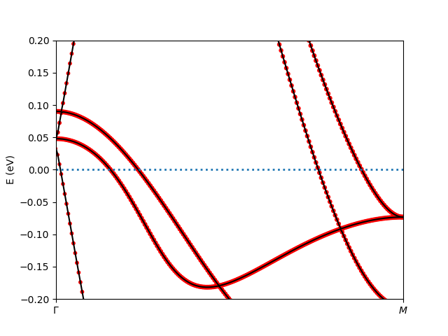
One can view the band structure in a fine energy window near Fermi level by typing:
$ cd lowh && ${COMRISB_BIN}/plot_band_tf.py -el -0.2 -eh 0.2 && cd ..
It generates the following band structure decorated with 3d-orbital weights.
This concludes the tutorial of ComRISB.
Further reference on this topic: [Zhang15] for experiment and [Choi19] for DMFT results.
P. Zhang, T. Qian, P. Richard, X. P. Wang, H. Miao, B. Q. Lv, B. B. Fu, T. Wolf, C. Meingast, X. X. Wu, Z. Q. Wang, J. P. Hu, and H. Ding, Observation of Two Distinct ${d}_{xz}$/${d}_{yz}$ Band Splittings in FeSe, Phys. Rev. B 91, 214503 (2015).
S. Choi, P. Semon, B. Kang, A. Kutepov, and G. Kotliar, ComDMFT: A Massively Parallel Computer Package for the Electronic Structure of Correlated-Electron Systems, Computer Physics Communications 244, 277 (2019).