ComRISB calculation of Fe
In this example, we will review the DFT-LDA calculations with the FlapwMBPT package, using \(\alpha\)-Fe as an example. DFT+GRISB calculations of the paramagnetic (PM) and ferromagnetic (FM) phase with ComRISB package will be demonstrated.
Time for this part: ~90 minutes.
DFT-LDA calculation of Fe
Starting with the directory 3_Fe, follow the steps below to finish the DFT-LDA calculations. Type:
$ mkdir -p dft && cd dft
$ # create files ini, kpath, and kpoints for FlapwMBPT calculation.
$ ${COMRISB_BIN}/../ComBin/cif2matdelab.py ../bcc.cif -k 3
$ # create your own job file and submit
$ # or directly run FlapwMBPT if convenient.
$ mpirun -np 2 ${COMRISB_BIN}/rspflapw.exe
After the default 40 iterations, the charge density converges at
charge density self-consistency= 0.8638399E-08,
And the DFT-LDA energy reaches
dft: ETOT F = -2541.074138668239 -2541.074855981326.
DFT+GRISB calculation of PM Fe with zero interaction
We will first perform a DFT+GRISB calculation with zero interaction, i.e., \(U=J=0\). The purpose is to demonstrate that it is exactly equivalent to LDA, and to facilitate the illustration of correlation effects on the spectral function at a later step.
Changing back to the directory 3_Fe, follow the steps below to finish the DFT+GRISB calculations with zero interaction. Type:
$ mkdir -p dftg/u0j0/lowh && cp bcc.cif dftg/u0j0/lowh/. && cd dftg/u0j0/lowh
$ ${COMRISB_BIN}/init_grisb.py -u eV -s 1
$ # -u eV: set internal energy unit to be eV.
$ # -s 1: set spin z-component order to be -1/2 to 1/2.
Following the screenshot below to specify the GRISB calculation. Press enter-key to make your choice:
structure info read from bcc.cif.

User inputs to initialize G-RISB simulation.
[?] Break spin-symmetry: no
 > no
   yes

[?] Break orbital-symmetry: crystal field effect
   no
 > crystal field effect
   full symmetry breaking

[?] Include spin-orbit coupling: no
 > no
   yes

[?] Parametrize Coulomb-matrix: Slater-Condo with [U,J]
 > Slater-Condo with [U,J]
   Slater-Condo with [F0,F2,...]
   Kanamori with [U,J]
   Manual input

[?] Coulomb double counting: FLL dc (updated at charge iter., Rec.)
 > FLL dc (updated at charge iter., Rec.)
   Fix dc potential
   FLL dc self-consistent
   No dc

[?] Solution of embedding Hamiltonian: VTED with Sz symmetry
   Valence truncation ED (VTED)
 > VTED with Sz symmetry
   VTED with S=0
   VTED with Jz symmetry
   ML (kernel-ridge)
   ML (normal-mode-1d)
   DMGR (expt.)
   ML (normal-mode-2d)
   ML (normal-mode-3d)
   HF (debugging only)

Equivalent atom indices:
    [0 0 0 1 1] means 0-2 and 3-4 are two sets of eq. atms.
[?] Equivalent atom indices: [0]
 > [0]
   modify


 ------------
 atom 0 Fe
[?] Is this atom correlated (Y/n):
[?] Correlated orbital: d
   s
   p
 > d
   f

[?] Enter U J(sep. by space, eV): 0 0
n_symm_ops = 48 from point-group analysis
           = 48 after screening.
correlated atom 0 with point group: Oh.
chi_space 0: 1 equivalent ireps
              (5, 3) basis vectors.
chi_space 1: 1 equivalent ireps
              (5, 2) basis vectors.
This finishes the manual initialization. Alternative ways for initialization will be touched in the next steps. Two new files are created: ginit.json and GParam.h5. ginit.json saves all the information for initialization in json format, and GParam.h5 is an input file for the GRISB calculation in hdf5 format. One can check the data structure by typing:
$ h5ls -r GParam.h5
The following information will be displayed on the screen:
/                        Group
/impurity_0              Group
/impurity_0/V2E          Dataset {10, 10, 10, 10}
/impurity_0/db2sab       Dataset {10, 10}
/impurity_0/lie_params   Dataset {2, 24, 3}
/impurity_0/lx           Dataset {10, 10}
/impurity_0/ly           Dataset {10, 10}
/impurity_0/lz           Dataset {10, 10}
/impurity_0/matrix_basis Dataset {2, 10, 10}
/impurity_0/sx           Dataset {10, 10}
/impurity_0/sy           Dataset {10, 10}
/impurity_0/symbol_matrix Dataset {10, 10}
/impurity_0/symm_operations_3d Dataset {48, 3, 3}
/impurity_0/symm_operations_csh Dataset {48
Use the followint command to view a specific dataset, for instance, the symbolic matrix for local self-energy structure simplified due to point group symmetry:
$ h5dump -d /impurity_0/symbol_matrix GParam.h5
The following information will be displayed on the screen:
HDF5 "GParam.h5" {
DATASET "/impurity_0/symbol_matrix" {
   DATATYPE  H5T_STD_I64LE
   DATASPACE  SIMPLE { ( 10, 10 ) / ( 10, 10 ) }
   DATA {
   (0,0): 1, 0, 0, 0, 0, 0, 0, 0, 0, 0,
   (1,0): 0, 1, 0, 0, 0, 0, 0, 0, 0, 0,
   (2,0): 0, 0, 1, 0, 0, 0, 0, 0, 0, 0,
   (3,0): 0, 0, 0, 1, 0, 0, 0, 0, 0, 0,
   (4,0): 0, 0, 0, 0, 1, 0, 0, 0, 0, 0,
   (5,0): 0, 0, 0, 0, 0, 1, 0, 0, 0, 0,
   (6,0): 0, 0, 0, 0, 0, 0, 2, 0, 0, 0,
   (7,0): 0, 0, 0, 0, 0, 0, 0, 2, 0, 0,
   (8,0): 0, 0, 0, 0, 0, 0, 0, 0, 2, 0,
   (9,0): 0, 0, 0, 0, 0, 0, 0, 0, 0, 2
   }
}
}
Specifically, here it shows a \(e_g-t_{2g}\) splitting.
To perform DFT+GRISB calculation, an additional input file comrisb.ini in text format is prepared in the upper directory u0j0. It is a simplified version of comdmft.ini for the DMFT calculation using ComSUITE package, which provides information for the construction of wannier interface by the ComWann module. The comrisb.ini reads, in this example, as:
control={
        'initial_dft_dir': '../../dft/',
        'method': 'lda+risb',
        'mpi_prefix': "mpirun -np 8",
        'max_iter_num_outer': 50,
        'impurity_problem': [[1, 'd']],
        'impurity_problem_equivalence': [1],
        }

wan_hmat={
        'froz_win_min': -10.0,
        'froz_win_max': 10.0,
        }
To run the DFT+GRISB calculation, execute the following command or prepare your job script accordingly and submit:
$ cd ..  # up to u0j0 folder
$ python3.7 ${COMRISB_BIN}/comrisb.py -c  # -c: continuous run
As expected, the job converges with one iteration. The file convergence.log records the convergence information:
i_outer    delta_rho            etot           mu    err_risb       min_z
---------  -----------  --------------  -----------  ----------  ----------
       0   0.00000001  -2541.07413883  -0.00000032  0.00000041  0.99999992
The total energy etot is the same as DFT-LDA result, and the kinetic energy renormalization factor is identity. The timing information is saved in file cmd.log.
Several local quantities of interest are occupations for \(t_{2g}\) and \(e_{g}\) orbitals, which can be obtained from lowh/GLog.h5 from the dataset /impurity_0/NC_PHY, or search for the last entries of ncp-renorm in lowh/Gutz.log:
************    ncp-renorm  ************
imp=  1
real part
  0.6769   0.0000   0.0000   0.0000   0.0000   0.0000   0.0000   0.0000   0.0000   0.0000
  0.0000   0.6769   0.0000   0.0000   0.0000   0.0000   0.0000   0.0000   0.0000   0.0000
  0.0000   0.0000   0.6769   0.0000   0.0000   0.0000   0.0000   0.0000   0.0000   0.0000
  0.0000   0.0000   0.0000   0.6769   0.0000   0.0000   0.0000   0.0000   0.0000   0.0000
  0.0000   0.0000   0.0000   0.0000   0.6769   0.0000   0.0000   0.0000   0.0000   0.0000
  0.0000   0.0000   0.0000   0.0000   0.0000   0.6769   0.0000   0.0000   0.0000   0.0000
  0.0000   0.0000   0.0000   0.0000   0.0000   0.0000   0.5996   0.0000   0.0000   0.0000
  0.0000   0.0000   0.0000   0.0000   0.0000   0.0000   0.0000   0.5996   0.0000   0.0000
  0.0000   0.0000   0.0000   0.0000   0.0000   0.0000   0.0000   0.0000   0.5996   0.0000
  0.0000   0.0000   0.0000   0.0000   0.0000   0.0000   0.0000   0.0000   0.0000   0.5996
  sub_tot=  6.459972  0.000000
Each \(t_{2g}\) orbital occupies 0.68 electrons, and 0.60 for each \(e_{g}\) orbital., with total 6.46 3d-electrons.
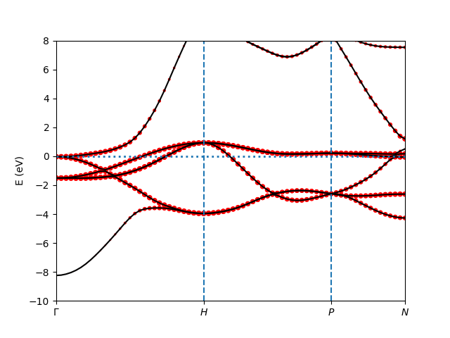
The band structure can be obtained by using the following script:
$ cd lowh && ${COMRISB_BIN}/plot_band_tf.py -el -10 -eh 8 && cd ..
It generates band structure decorated with 3d-orbital weights.
DFT+GRISB calculation of PM Fe
One way to set up the calculation is create a new directory u5j0.8 and repeat the above procedure with the correct nonzero interaction parameters. Here we introduce an alternative easier way by simply modifying the parameters with provided scripts. Starting with directory u0j0, type:
$ cd ../ && cp -r u0j0 u5j0.8 && cd u5j0.8/lowh/
$ ${COMRISB_BIN}/switch_gparam.py --unique_u_ev 5 --unique_j_ev 0.8
Now we can start the calculation as previously:
$ cd ..  # up to u5j0.8 folder
$ python3.7 ${COMRISB_BIN}/comrisb.py -c
It will take 16 iterations to converge, with the convergence.log file:
i_outer    delta_rho            etot           mu     err_risb       min_z
-------  -----------  --------------  -----------  -----------  ----------
      0   0.00189709  -2540.91218004   0.06088410   0.00000009  0.81693596
      1   0.00043149  -2540.91474874   0.06088307  -0.00000123  0.81693593
      2   0.00004852  -2540.91473052  -0.01841208   0.00000072  0.81961856
      3   0.00004149  -2540.91421012  -0.05360858  -0.00071526  0.82078603
      4   0.00001536  -2540.91411466  -0.05859637  -0.00000040  0.82093853
      5   0.00000442  -2540.91416410  -0.05392061  -0.00000404  0.82078284
      6   0.00000217  -2540.91421368  -0.05114723  -0.00000065  0.82068645
      7   0.00000129  -2540.91422747  -0.05094792   0.00000524  0.82067366
      8   0.00000077  -2540.91422652  -0.05156255  -0.00000480  0.82070242
      9   0.00000044  -2540.91422601  -0.05202869   0.00000124  0.82071461
     10   0.00000026  -2540.91410120  -0.05186064  -0.00048290  0.82116617
     11   0.00000012  -2540.91421954  -0.05225935  -0.00000312  0.82072632
     12   0.00000007  -2540.91422142  -0.05217349   0.00000491  0.82071604
     13   0.00000004  -2540.91422139  -0.05227547   0.00000274  0.82072138
     14   0.00000002  -2540.91421786  -0.05236450   0.00000157  0.82072514
     15   0.00000001  -2540.91422034  -0.05241289   0.00000587  0.82072286
     16   0.00000001  -2540.91420773  -0.05241025  -0.00000471  0.82072818
The updated local orbital occupations due to correlation can be read from the lowh/Gutz.log file:
************    ncp-renorm  ************
imp=  1
real part
  0.6792   0.0000   0.0000   0.0000   0.0000   0.0000   0.0000   0.0000   0.0000   0.0000
  0.0000   0.6792   0.0000   0.0000   0.0000   0.0000   0.0000   0.0000   0.0000   0.0000
  0.0000   0.0000   0.6792   0.0000   0.0000   0.0000   0.0000   0.0000   0.0000   0.0000
  0.0000   0.0000   0.0000   0.6792   0.0000   0.0000   0.0000   0.0000   0.0000   0.0000
  0.0000   0.0000   0.0000   0.0000   0.6792   0.0000   0.0000   0.0000   0.0000   0.0000
  0.0000   0.0000   0.0000   0.0000   0.0000   0.6792   0.0000   0.0000   0.0000   0.0000
  0.0000   0.0000   0.0000   0.0000   0.0000   0.0000   0.5936   0.0000   0.0000   0.0000
  0.0000   0.0000   0.0000   0.0000   0.0000   0.0000   0.0000   0.5936   0.0000   0.0000
  0.0000   0.0000   0.0000   0.0000   0.0000   0.0000   0.0000   0.0000   0.5936   0.0000
  0.0000   0.0000   0.0000   0.0000   0.0000   0.0000   0.0000   0.0000   0.0000   0.5936
  sub_tot=  6.449706  0.000000
In this example, correlation effects introduce very small modification to the orbital occupations.
The kinetic energy renormalization matrix \(Z=R^\dagger R\) can be retrieved from lowh/GLog.h5 as the dataset /impurity_0/R, or from lowh/Gutz.log file:
************     z-out-sym  ************
imp=  1
real part
  0.8799   0.0000   0.0000   0.0000   0.0000   0.0000   0.0000   0.0000   0.0000   0.0000
  0.0000   0.8799   0.0000   0.0000   0.0000   0.0000   0.0000   0.0000   0.0000   0.0000
  0.0000   0.0000   0.8799   0.0000   0.0000   0.0000   0.0000   0.0000   0.0000   0.0000
  0.0000   0.0000   0.0000   0.8799   0.0000   0.0000   0.0000   0.0000   0.0000   0.0000
  0.0000   0.0000   0.0000   0.0000   0.8799   0.0000   0.0000   0.0000   0.0000   0.0000
  0.0000   0.0000   0.0000   0.0000   0.0000   0.8799   0.0000   0.0000   0.0000   0.0000
  0.0000   0.0000   0.0000   0.0000   0.0000   0.0000   0.8207   0.0000   0.0000   0.0000
  0.0000   0.0000   0.0000   0.0000   0.0000   0.0000   0.0000   0.8207   0.0000   0.0000
  0.0000   0.0000   0.0000   0.0000   0.0000   0.0000   0.0000   0.0000   0.8207   0.0000
  0.0000   0.0000   0.0000   0.0000   0.0000   0.0000   0.0000   0.0000   0.0000   0.8207
imp=  1 eigen values of         z:
   0.8799    0.8799    0.8799    0.8799    0.8799    0.8799    0.8207    0.8207    0.8207    0.8207
The Z-factor for \(t_{2g}\) and \(e_g\) orbital reduces from identity to 0.88 and 0.82 respectively.
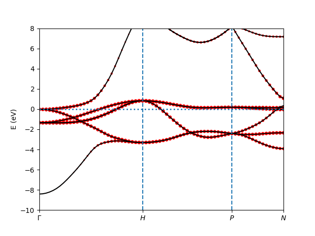
The Gutzwiller quasi-particle band structure can be obtained by using the same script as previously:
$ cd lowh && ${COMRISB_BIN}/plot_band_tf.py -el -10 -eh 8 && cd ..
It generates band structure decorated with 3d-orbital weights.
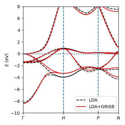
To contrast the DFT+GRISB band structure of Fe with DFT-LDA results obtained earlier, type:
$ cd ../figure1 && python plot.py && cd ../u5j0.8
and one obtained the following figure.
DFT+GRISB calculation of FM Fe with screened interaction
In the previous step, we performed a DFT+GRISB calculation for Fe with interaction parameters U=5 eV and J=0.8 eV. There another FM solution of lower energy to be explored. It can be investigated by a initial guess of the GRISB nonlinear equation solution with FM-type spin symmetry breaking. Note that the exchange-correlation energy is still spin-symmetric LDA, the energy gain is therefore purely from the onsite screened interactions.
To prepare the FM calculation, we follow the previous step to create a new folder u5j0.8_fm. Type:
$ cd .. && cp -r u5j0.8 u5j0.8_fm && cd u5j0.8_fm/lowh
To introduce an initial guess for the FM solution, we rerun the init_grisb.py script. However, since the file ginit.json already exists, the script will directly read informatin there without explicitly asking any questions. This will simply regenerate the input file GParam.h5 for PM GRISB calculation. To introduce spin symmetry breaking, one could delete ginit.json and answer questions properly while running init_grisb.py. We take another easier route by editing the ginit.json file, and reinitialize. Type the fillowing command to replace the value of 1 by 2 for spin-symmetry breaking:
$ sed -i 's/"ispin": 1/"ispin": 2/' ginit.json
$ ${COMRISB_BIN}/init_grisb.py -u eV -s 1
Further information about how the spin symmetry is to be broken needs to be provided through the script init_magnetism.py:
$ ${COMRISB_BIN}/init_magnetism.py
and choose the following as below:
[?] choose unit used in CyGutz calculation: eV (1)
   Rydberg (13.6)
 > eV (1)

[?] which way to apply vext: initial step only
 > initial step only
   all iterations

 total 1 impurities with equivalence indices
 [0]

 impurity 0
[?] enter field direction x y z seperated by space. (e.g., 0 0 1): 0 0 1
[?] enter b field magnitude (eV/Bohr magneton): 0.3
 maximal symmetrization error of vext = 2.22e-16
Final step for preparation, delete the file GLog.h5 if present, as it save the PM solution:
$ rm -f GLog.h5
Now the FM calculation can be started as previously:
$ cd ..  # up to u5j0.8_fm folder
$ python3.7 ${COMRISB_BIN}/comrisb.py -c
The job converges with 13 iterations. The convergence.log reads like:
i_outer    delta_rho            etot           mu     err_risb       min_z
--------  -----------  --------------  -----------  -----------  ----------
      0   0.00005456  -2540.93820420  -0.10544984  -0.00000539  0.89580499
      1   0.00001433  -2540.93846530  -0.10545215   0.00000255  0.89580387
      2   0.00000205  -2540.93842080  -0.11472259  -0.00000066  0.89596959
      3   0.00000075  -2540.93837572  -0.11994221  -0.00018106  0.89610887
      4   0.00000053  -2540.93837535  -0.12176499  -0.00000070  0.89607918
      5   0.00000040  -2540.93839476  -0.12246404  -0.00000350  0.89608366
      6   0.00000027  -2540.93840743  -0.12315630  -0.00000035  0.89609038
      7   0.00000016  -2540.93841304  -0.12387580  -0.00000278  0.89609854
      8   0.00000010  -2540.93841516  -0.12449917  -0.00000282  0.89610619
      9   0.00000006  -2540.93841626  -0.12498324  -0.00000048  0.89611241
     10   0.00000004  -2540.93841692  -0.12535097   0.00000165  0.89611723
     11   0.00000002  -2540.93841800  -0.12563217  -0.00000496  0.89611977
     12   0.00000001  -2540.93841819  -0.12585449  -0.00000178  0.89612259
     13   0.00000001  -2540.93841838  -0.12602852  -0.00000106  0.89612503
The total energy reduces from -2540.9142 Ry in PM phase to -2540.9384 in the FM phasse. The Z-factor generally increase with symmetry breaking. The magnetic moment, as can be located as total magnetic moment: in the lowh/Gutz.log file, is \(2.14 \mu_B\), comparable the experimental result \(2.22 \mu_B\).
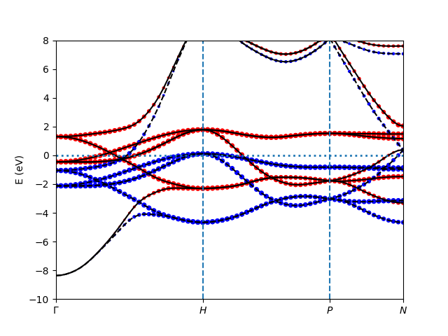
The FM band structure can be calculated as previously:
$ cd lowh && ${COMRISB_BIN}/plot_band_tf.py -el -10 -eh 8 && cd ..
It generates band structure decorated with 3d-orbital weights.
This concludes the tutorial of DFT+GRISB calculations of PM and FM phase using ComRISB package.
Further reading on this topic: [Deng08], [Lanata13], [Borghi14], [Schickling16].
X. Y. Deng, X. Dai, and Z. Fang, LDA+Gutzwiller Method for Correlated Electron Systems, EPL (Europhysics Letters) 83, 37008 (2008).
N. Lanata, H. U. R. Strand, G. Giovannetti, B. Hellsing, L. de Medici, and M. Capone, Orbital Selectivity in Hund’s Metals: The Iron Chalcogenides, Phys. Rev. B 87, 045122 (2013).
G. Borghi, M. Fabrizio, and E. Tosatti, Gutzwiller Electronic Structure Calculations Applied to Transition Metals: Kinetic Energy Gain with Ferromagnetic Order in Bcc Fe, Phys. Rev. B 90, 125102 (2014).
T. Schickling, J. Bünemann, F. Gebhard, and L. Boeri, Quasiparticle Bands and Structural Phase Transition of Iron from Gutzwiller Density-Functional Theory, Phys. Rev. B 93, 205151 (2016).